Tutorial

Go through few examples.

First, import the following dependencies that we will be work with.

import numpy as np
from signal_design import Axis, Relation, Signal, Spectrum
import matplotlib.pyplot as plt 

Matplotlib is building the font cache; this may take a moment.

---------------------------------------------------------------------------
KeyboardInterrupt                         Traceback (most recent call last)
Cell In[1], line 3
      1 import numpy as np
      2 from signal_design import Axis, Relation, Signal, Spectrum
----> 3 import matplotlib.pyplot as plt 

File ~/checkouts/readthedocs.org/user_builds/signal-design/envs/latest/lib/python3.11/site-packages/matplotlib/pyplot.py:52
     50 from cycler import cycler
     51 import matplotlib
---> 52 import matplotlib.colorbar
     53 import matplotlib.image
     54 from matplotlib import _api

File ~/checkouts/readthedocs.org/user_builds/signal-design/envs/latest/lib/python3.11/site-packages/matplotlib/colorbar.py:19
     16 import numpy as np
     18 import matplotlib as mpl
---> 19 from matplotlib import _api, cbook, collections, cm, colors, contour, ticker
     20 import matplotlib.artist as martist
     21 import matplotlib.patches as mpatches

File ~/checkouts/readthedocs.org/user_builds/signal-design/envs/latest/lib/python3.11/site-packages/matplotlib/contour.py:13
     11 import matplotlib as mpl
     12 from matplotlib import _api, _docstring
---> 13 from matplotlib.backend_bases import MouseButton
     14 from matplotlib.text import Text
     15 import matplotlib.path as mpath

File ~/checkouts/readthedocs.org/user_builds/signal-design/envs/latest/lib/python3.11/site-packages/matplotlib/backend_bases.py:45
     42 import numpy as np
     44 import matplotlib as mpl
---> 45 from matplotlib import (
     46     _api, backend_tools as tools, cbook, colors, _docstring, text,
     47     _tight_bbox, transforms, widgets, get_backend, is_interactive, rcParams)
     48 from matplotlib._pylab_helpers import Gcf
     49 from matplotlib.backend_managers import ToolManager

File ~/checkouts/readthedocs.org/user_builds/signal-design/envs/latest/lib/python3.11/site-packages/matplotlib/text.py:16
     14 from . import _api, artist, cbook, _docstring
     15 from .artist import Artist
---> 16 from .font_manager import FontProperties
     17 from .patches import FancyArrowPatch, FancyBboxPatch, Rectangle
     18 from .textpath import TextPath, TextToPath  # noqa # Logically located here

File ~/checkouts/readthedocs.org/user_builds/signal-design/envs/latest/lib/python3.11/site-packages/matplotlib/font_manager.py:1551
   1547     _log.info("generated new fontManager")
   1548     return fm
-> 1551 fontManager = _load_fontmanager()
   1552 findfont = fontManager.findfont
   1553 get_font_names = fontManager.get_font_names

File ~/checkouts/readthedocs.org/user_builds/signal-design/envs/latest/lib/python3.11/site-packages/matplotlib/font_manager.py:1545, in _load_fontmanager(try_read_cache)
   1543             _log.debug("Using fontManager instance from %s", fm_path)
   1544             return fm
-> 1545 fm = FontManager()
   1546 json_dump(fm, fm_path)
   1547 _log.info("generated new fontManager")

File ~/checkouts/readthedocs.org/user_builds/signal-design/envs/latest/lib/python3.11/site-packages/matplotlib/font_manager.py:1017, in FontManager.__init__(self, size, weight)
   1014 for path in [*findSystemFonts(paths, fontext=fontext),
   1015              *findSystemFonts(fontext=fontext)]:
   1016     try:
-> 1017         self.addfont(path)
   1018     except OSError as exc:
   1019         _log.info("Failed to open font file %s: %s", path, exc)

File ~/checkouts/readthedocs.org/user_builds/signal-design/envs/latest/lib/python3.11/site-packages/matplotlib/font_manager.py:1044, in FontManager.addfont(self, path)
   1042     self.afmlist.append(prop)
   1043 else:
-> 1044     font = ft2font.FT2Font(path)
   1045     prop = ttfFontProperty(font)
   1046     self.ttflist.append(prop)

KeyboardInterrupt: 

Contents:

1. Introduction

2. Axis

3. Relation

4. Signal

5. Spectrum

6. Overriding methods

1. Introduction

The project was created for a simple design of signals. Easy and fast way to create signals. But to create a new one, we have developed a some new entities that help in creating of signals.

Below representation structure of this objects in a project.

Following this diagram, we describe how to work with the library signal-design.

2. Axis

We should define the number of axis elements (size) in order to create a new instances of Axis. Size should be positive integer. By default sample is equal to 1, start of axis is 0 and end of axis is not define (equal None). You can changer them.

# An example of axis with sample 1 and start 0.
axis_1 = Axis(11)

# An example of axis with sample 0.5 and start 0.
axis_2 = Axis(11, 0.5)

# An example of axis with sample 0.5 and start 1.
axis_3 = Axis(11, 0.5, 1.)

Properties of axis can be changed.

print(f"Before:\n{axis_3}")
axis_3.size = 5
print(f"After:\n{axis_3}")

Before:
size: 11
sample: 0.5
start: 1.0
end: None

After:
size: 5
sample: 0.5
start: 1.0
end: None

If the end value was not specified when the instance was created, then when it is requested, it will be obtained by multiplying the number of samples minus one by the sample and summing from the start value. And it remains recorded.

print(f"End of axis: {axis_3.end}")
print(f"Axis params:\n{axis_3}")

End of axis: 3.0
Axis params:
size: 5
sample: 0.5
start: 1.0
end: 3.0

Changing one of the three parameters: size, sample or start will change the end value of axis to undefined (None).

axis_3.start = 2.
print(axis_3)

size: 5
sample: 0.5
start: 2.0
end: None

If we have a start, sample and size, then it is not difficult to determine the end value of the axis. But it is not always possible to get the exact end value or the exact value of the sample. For example, when the sampling step cannot be represented by a decimal number. For example, 1/3.

Below is an example representation of a sequence from 0 to 10 with 4 samples.

result = np.linspace(0, 10, 4)
print(result)
print(np.diff(result))
print(np.diff(np.diff(result)))

[ 0.          3.33333333  6.66666667 10.        ]
[3.33333333 3.33333333 3.33333333]
[ 0.0000000e+00 -4.4408921e-16]

As can be seen above, the discretization step cannot be represented exactly, then in this case, you can use the definition of the end value of the axis.

axis = Axis(4, 10/3, 0, 10)
print(axis.array)

[ 0.          3.33333333  6.66666667 10.        ]

The array property of the Axis class uses the get_array function, which uses the np.linspace function to get the np.ndarray sequence. At the end is an example of how to change the get_array function if you are not satisfied with finding the np.ndarray sequence.

The Axis class does not check which sampling step and the number of samples in a given interval or the final value of the interval. Due to the inaccuracy of determining one of the parameters. Thus, a situation is possible when the sampling step does not correspond to the number of samples. And the result will depend on the parameters that a certain method uses. See the documentation for details.

axis = Axis(4, 10/3, 0, 10)
print(f"Before:\n{axis.array}")
print(f"sample: {axis.sample}")
axis.end = 1000
print(f"After:\n{axis.array}")
print(f"smaple: {axis.sample}")

Before:
[ 0.          3.33333333  6.66666667 10.        ]
sample: 3.3333333333333335
After:
[   0.          333.33333333  666.66666667 1000.        ]
smaple: 3.3333333333333335

To avoid such situations, it is desirable to use the exact number of samples in a given interval for a given discretization.

axis = Axis(101, 0.1, -1)
print(f"Axis info:\n{axis}")
print(f"End of axis: {axis.end}")
print(f"Array axis:\n{axis.array}")

Axis info:
size: 101
sample: 0.1
start: -1
end: None

End of axis: 9.0
Array axis:
[-1.  -0.9 -0.8 -0.7 -0.6 -0.5 -0.4 -0.3 -0.2 -0.1  0.   0.1  0.2  0.3
  0.4  0.5  0.6  0.7  0.8  0.9  1.   1.1  1.2  1.3  1.4  1.5  1.6  1.7
  1.8  1.9  2.   2.1  2.2  2.3  2.4  2.5  2.6  2.7  2.8  2.9  3.   3.1
  3.2  3.3  3.4  3.5  3.6  3.7  3.8  3.9  4.   4.1  4.2  4.3  4.4  4.5
  4.6  4.7  4.8  4.9  5.   5.1  5.2  5.3  5.4  5.5  5.6  5.7  5.8  5.9
  6.   6.1  6.2  6.3  6.4  6.5  6.6  6.7  6.8  6.9  7.   7.1  7.2  7.3
  7.4  7.5  7.6  7.7  7.8  7.9  8.   8.1  8.2  8.3  8.4  8.5  8.6  8.7
  8.8  8.9  9. ]

There are situations when you know the initial value, the sampling step and the final value. In order not to count the number of samples, you can use the static method Axis.get_using_end.

Let’s create time axis. Start time is 0. end time is 10. sample of array 0.001

axis = Axis.get_using_end(start=0., end=10., sample=0.001)
print(f"Axis 1:\n{axis}")

axis_2 = Axis.get_using_end(0.0, 0.25, 0.1, False)
print(f"Axis 2:\n{axis_2}")
print(f"End of Axis 2: {axis_2.end}")

Axis 1:
size: 10001
sample: 0.001
start: 0.0
end: 10.0

Axis 2:
size: 3
sample: 0.1
start: 0.0
end: None

End of Axis 2: 0.2

The important feature is the number of samples per axis, then the sampling step is next in importance, and then the start of the axis. The final value has less meaning and is only used by some methods. But when they are defined exactly, the desired correct result can be obtained.

3. Relation

A relation instance is a representation of some mathematical functions, such as y = f(x).

Look at building simple function of sin with frequency 1 Hz.

time = Axis.get_using_end(0., 10., 0.01)
amplitude = np.sin(2*np.pi*time.array)
sin_1 = Relation(time, amplitude)

sin_1- instance of class Relation represent dependencies between time and amplitude such as mathematical function

\[ amplitude = sin(2\cdot\pi\cdot time) \]

Relation instance have same properties as ArrayAxis. Also have other properties: x, y.

We can use matplotlib to show result in next section.

r_time, r_amplitude = sin_1.get_data()
plt.plot(r_time, r_amplitude)
plt.xlabel('Time, s')
plt.ylabel('Amplitude')
plt.title('Sin 1Hz')

Text(0.5, 1.0, 'Sin 1Hz')

Also you can find maximum and minimum of relation

print(sin_1.max())
print(sin_1.min())

1.0
-1.0

Norm of function.

sin_1.get_norm()

500.0

Interpolate of function expected by instance of Relation using new array axis

time_new = Axis.get_using_end(0.,10., 0.0005)
interpolate_sin_1 = sin_1.interpolate_extrapolate(time_new)

Shift relation, equal y=f(x+c) where c - is shift constant.

shifted_sin_1 = sin_1.shift(2)

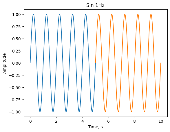
Also you can select interesting segment of data using to methods, select_data method or use square brackets.

r_time, r_amplitude = sin_1.get_data()
plt.plot(*sin_1.select_data(0., 5.).get_data())
plt.plot(*sin_1[5.:10.].get_data())
plt.xlabel('Time, s')
plt.ylabel('Amplitude')
plt.title('Sin 1Hz')

Text(0.5, 1.0, 'Sin 1Hz')

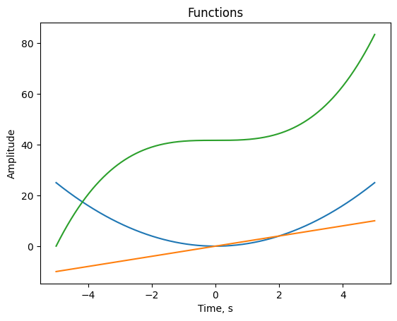
cumulative integration and differentiation of function

time_5 = Axis.get_using_end(-5., 5., 0.001)
y2 = Relation(time_5, time_5.array**2)
diff_y2 = y2.diff()
integration_y2 = y2.integrate()

plt.plot(*y2.get_data())
plt.plot(*diff_y2.get_data())
plt.plot(*integration_y2.get_data())
plt.xlabel('Time, s')
plt.ylabel('Amplitude')
plt.title('Functions')

Text(0.5, 1.0, 'Functions')

exponent of function. $\( y = f(x) \)\( \)\( r = e^y \)$ equal:

r = sin_1.exp()

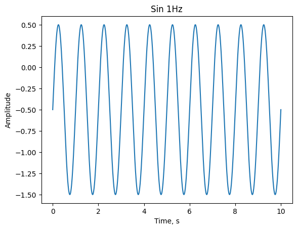
With instance of class Relation we can use different mathematical operations (+, -, *, /, **, +=, -=, /=, *=). Operation can be with other instance of class Relation or numbers. Next examples with number. Subtraction constant from sin_1.

sub_sin_1 = sin_1-0.5
plt.plot(*sub_sin_1.get_data())
plt.xlabel('Time, s')
plt.ylabel('Amplitude')
plt.title('Sin 1Hz')

Text(0.5, 1.0, 'Sin 1Hz')

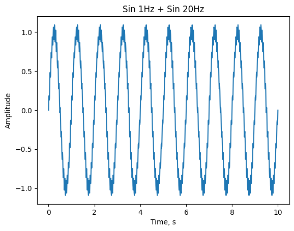
To demonstrate operation with other Relation instance, let’s create other sin function with 20Hz. And summing two instances sin_1 and sin_20.

sin_20 = Relation(time, 0.1*np.sin(time.array*2*np.pi*20))
sum_sin1_sin20 = sin_1 + sin_20

r_time_1_20, r_amplitude_1_20 = sum_sin1_sin20.get_data()
plt.plot(r_time_1_20, r_amplitude_1_20)
plt.xlabel('Time, s')
plt.ylabel('Amplitude')
plt.title('Sin 1Hz + Sin 20Hz')

Text(0.5, 1.0, 'Sin 1Hz + Sin 20Hz')

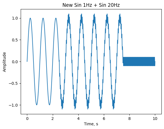
It’s better if you use a Relation instance with an equal axis array, but sometimes you can’t use. Then, when calculating math operation, new array axis found small sample and big boundaries. And y component of each relation interpolate with new common axis and extrapolate by zeros. After that, execute mathematical operation and return the result.

time1 = Axis.get_using_end(0., 7.5, 0.005)
time2 = Axis.get_using_end(2.5, 10., 0.001)

new_sin_1 = Relation(time1, np.sin(time1.array*2*np.pi))
new_sin_20 = Relation(time2, 0.1*np.sin(time2.array*2*np.pi*20))

new_sum_sin1_sin20 = new_sin_1 + new_sin_20

plt.plot(*new_sum_sin1_sin20.get_data())
plt.xlabel('Time, s')
plt.ylabel('Amplitude')
plt.title('New Sin 1Hz + Sin 20Hz')

Text(0.5, 1.0, 'New Sin 1Hz + Sin 20Hz')

To find two common axis for relations use class method equalize. This method use for math operations, convolution and correlations.

common_new_sin_1, common_new_sin_20 = Relation.equalize(new_sin_1, new_sin_20)

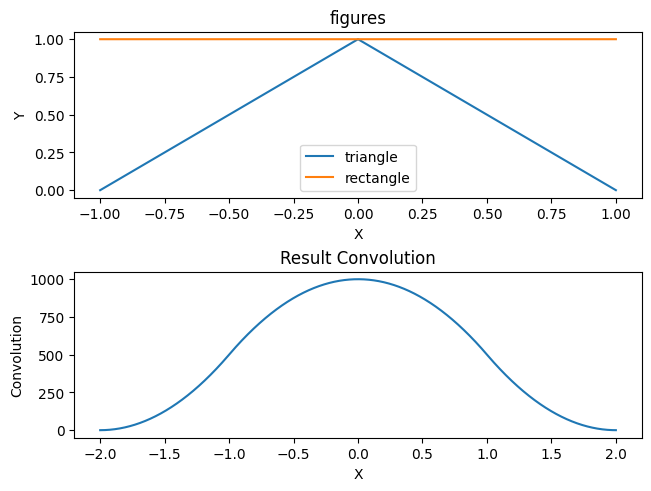
Available class methods to correlate and convolve. Look on convolution triangle and rectangle.

x = Axis.get_using_end(-1., 1., 0.001)

triangle = Relation(x, -1*(np.abs(x.array)-1))
rectangle = Relation(x, np.ones(x.size))

convolution = Relation.convolve(triangle, rectangle)

figure, axis = plt.subplots(2, 1, constrained_layout=True)

axis[0].plot(*triangle.get_data(), label='triangle')
axis[0].plot(*rectangle.get_data(), label='rectangle')
axis[0].set_title("figures")
axis[0].set_xlabel("X")
axis[0].set_ylabel("Y")
axis[0].legend()


axis[1].plot(*convolution.get_data())
axis[1].set_xlabel('X')
axis[1].set_ylabel('Convolution')
axis[1].set_title('Result Convolution')

Text(0.5, 1.0, 'Result Convolution')

4. Signal

The class Signal inherited from the class Relation. It has the same operation as Relation class. Additional has operation to convert signal to spectrum.

List additional methods:

signal_sin_1 = Signal(sin_1)
signal_sin_1.get_spectrum()
signal_sin_1.get_amplitude_spectrum()
signal_sin_1.get_phase_spectrum()
signal_sin_1.get_reverse_signal()
signal_sin_1.add_phase(signal_sin_1)
signal_sin_1.sub_phase(signal_sin_1)

<signal_design.signal.Signal at 0x7f03dff0bd10>

and has properties: time and amplitude

print(signal_sin_1.time)
print(signal_sin_1.amplitude)

size: 1001
sample: 0.01
start: 0.0
end: 10.0

[ 0.00000000e+00  6.27905195e-02  1.25333234e-01 ... -1.25333234e-01
 -6.27905195e-02 -2.44929360e-15]

Let’s check that the sum of sin 1 Hz and 20 Hz has an amplitude spectrum of 1 Hz and 20 Hz.

signal_sum_sin1_sin20 = Signal(sum_sin1_sin20)
plt.plot(*signal_sum_sin1_sin20.get_amplitude_spectrum()[0:50].get_data())
plt.xlabel('Frequency, Hz')
plt.ylabel('Amplitude')
plt.title('Amplitude spectrum Sin 1Hz + Sin 20Hz')

Text(0.5, 1.0, 'Amplitude spectrum Sin 1Hz + Sin 20Hz')

Where an operation with signal is expected, the spectrum instance will be converted to signal instance and operation will be with them.

5. Spectrum

The Spectrum class inherited from Relation class. It has the same operation as Relation class. Additional has operation to convert spectrum to signal.

List additional methods:

spectrum_sum_sin1_sin20 = signal_sum_sin1_sin20.get_spectrum()
spectrum_sum_sin1_sin20.get_amplitude_spectrum()
spectrum_sum_sin1_sin20.get_phase_spectrum()
spectrum_sum_sin1_sin20.get_reverse_filter()
spectrum_sum_sin1_sin20.add_phase(spectrum_sum_sin1_sin20)
spectrum_sum_sin1_sin20.sub_phase(spectrum_sum_sin1_sin20)

<signal_design.spectrum.Spectrum at 0x7f03df652050>

Class method get_spectrum_from_amplitude_phase

amplitude_spectrum = spectrum_sum_sin1_sin20.get_amplitude_spectrum()
phase_spectrum = spectrum_sum_sin1_sin20.get_phase_spectrum()

spectrum = Spectrum.get_from_amplitude_phase(amplitude_spectrum, phase_spectrum)

Where an operation with spectrum is expected, the signal instance will be converted to spectrum instance and operation will be with them.

6. Overriding methods

If the execution of any method of any class does not satisfy, then you can redefine it to the desired function before using it. The main thing is that the signature of the new function matches the old method.

The following are examples for the methods of the Axis class. Both for normal methods and for static ones.

def new_get_array(axis: Axis):
    return np.ones(axis.size)
Axis.get_array = new_get_array

axis = Axis.get_using_end(0, 10, 1)
print(axis.array)

[1. 1. 1. 1. 1. 1. 1. 1. 1. 1. 1.]

from signal_design.help_types import ArrayLike

def new_get_axis_from_array(array: ArrayLike):
    return Axis(2)
Axis.get_from_array = new_get_axis_from_array

axis = Axis.get_from_array([-1.0, -0.5, 0, 0.5])
print(axis)

size: 2
sample: 1
start: 0
end: None